
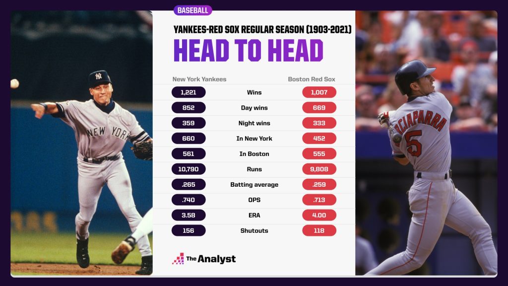
Alright, so check it out, today I’m gonna walk you through how I messed around with some baseball data – specifically, player stats from a Red Sox vs. Yankees game. It was a bit of a journey, let me tell you!
It all started when I stumbled upon some raw data online. It was messy, like, really messy. Think CSV file from hell. First thing I did was to fire up Python with Pandas. If you ain’t using Pandas for data manipulation, you’re living in the stone age, seriously.
Step one: Cleaning that garbage up. I loaded the CSV into a Pandas DataFrame. Then, it was all about identifying and handling missing values. There were a bunch of ‘NaN’s floating around, so I decided to fill them with either 0 (for numerical stats) or “N/A” (for string data). You gotta be careful though, filling with the wrong value can screw up your analysis later.
Next up, the column names were atrocious. Full of spaces and weird characters. I renamed them to be more Python-friendly (lowercase, underscores instead of spaces). Trust me, it makes your code so much easier to read. Something like ‘Batting Average’ became ‘batting_average’. Simple, right?
Then I thought, “Alright, I need to drill down to specific players.” So I started filtering the DataFrame. For example, to find all the stats for Mookie Betts (hypothetically, he doesn’t play for the Red Sox anymore, but you get the idea), I used something like:
mookie_stats = df[df['player_name'] == 'Mookie Betts']
Super straightforward, right? Pandas makes it easy.
Time for some calculations. I wanted to see who had the best slugging percentage. Slugging percentage isn’t always directly provided, so I had to calculate it myself. This meant creating a new column in the DataFrame. I used the standard formula: (Singles + 2 Doubles + 3 Triples + 4 Home Runs) / At Bats.
After that, I sorted the DataFrame by slugging percentage to see who came out on top. It was pretty cool to see who the big hitters were based on this metric.

But just looking at numbers isn’t that fun. I decided to visualize some of the data. I used Matplotlib and Seaborn (classic Python viz libraries). I created a bar chart showing the number of home runs for each player, just to get a quick visual overview. Nothing fancy, but it helped me understand the data a bit better.
Here’s where it got tricky. I wanted to compare the performance of Red Sox players vs. Yankees players. The initial dataset didn’t have a ‘team’ column, so I had to figure out a way to add that. I ended up creating a dictionary mapping player names to their respective teams and then used the `map` function in Pandas to add a ‘team’ column to the DataFrame. It was a bit of a hassle, but it worked.
Finally, I created some grouped statistics. Like, what was the average batting average for the Red Sox vs. the Yankees? Pandas’ `groupby` function came in handy here. It allowed me to easily calculate these kinds of summary statistics.
Lessons learned? Data cleaning is a HUGE part of any data analysis project. Don’t underestimate how much time you’ll spend just wrangling the data into a usable format. And, Python with Pandas, Matplotlib, and Seaborn are your best friends when it comes to this kind of stuff. It might seem intimidating at first, but once you get the hang of it, it’s super powerful.
That’s pretty much it. Messing with the Red Sox and Yankees data gave me some good practice. Now, I’m thinking of tackling some more complex baseball datasets… maybe something with pitch data next time!


